SAF Skyrmions - Micromagnetics

To simulate a SAF configuration, we use the UberMag python package. Then we import

discretisedfield, micromagneticmodel, oommfc for the micromagnetic simulation
functools, matplotlib.pyplot as auxiliar tools

import discretisedfield as df
import micromagneticmodel as mm
import oommfc as oc
import functools
import matplotlib.pyplot as plt

Initial Conditions¶

Lets first define what structure is going to be used. The mesh has

Region with three layers, where the spacer is the middle one with zero magnetization.
The sides of the mesh has the size of the diameter $D$ of the initial magnetization disk.
The spacer layer has a 2 nm height, while the ferromagnetic layers have 10 nm height.

def get_mesh(D:float):

    r = D/2
    p1 = (-r, -r, 0)
    p2 = (r, r, 22e-9)

    region = df.Region(p1=p1,p2=p2)
    subregions = {
        "bottom": df.Region(
            p1=p1,
            p2=(r, r, 10e-9)
        ),
        "spacer": df.Region(
            p1=(-r, -r, 10e-9),
            p2=(r, r, 12e-9)
        ),
        "top": df.Region(
            p1=(-r, -r, 12e-9),
            p2=(r, r, 22e-9)
        )
    }

    mesh = df.Mesh(
        region=region,
        cell=(3e-9, 3e-9, 1e-9),
        subregions=subregions
    )

    return mesh

D = 300e-9 # m
mesh1 = get_mesh(D)
mesh1.mpl.subregions(figsize=(18,6), filename='../images/notebooks/mesh_subregions.png')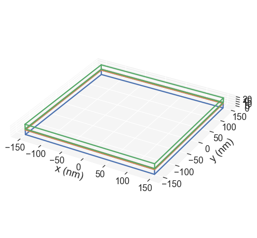

Magnetization¶

Now, we want to set the initial conditions for the magnetization:

Inner disk of diameter $d=40$ nm where the magnetization is antiparallel to outside of the disk.
Opposite directions for the top and bottom layers.

def Ms_init(pos, Ms, D):
    x, y, z = pos
    r = D/2
    if (x**2+y**2)**0.5 < r:
        if z < 10e-9:
            return -Ms
        else:
            return Ms
    else:
        return 0

def m_init(pos, d):
    x, y, z = pos
    r = d/2
    if (x**2+y**2)**0.5 < r:
        return (0, 0, -1)
    else:
        return (0, 0, 1)

d = 40e-9 # m
Ms = 380e3 # A/m

Ms_fun = functools.partial(Ms_init, Ms=Ms, D=D)
m_fun = functools.partial(m_init, d=d)

Parameters¶

We define some paramters to use in the simulation to replicate some of the results from Batistel & Brandão (2023). There are two important energy terms related to SAF Skyrmions:

DMI Interaction: Here it is important if using UberMag, to have it installed via conda cuz the official release doesnt include the extension DMI $C_{nv}$
RKKY Interaction: UberMag its capable of simulating the RKKY interaction with OOMMF as the backend, so no problem here.

# CONSTANTS
A = 1e-11 # J/m
sigma = -0.3e-3 # J/m^2 
K = 0.1e6 # J/m^3
dmi = 0.5e-3 # J/m^2

Once defined the constants, we initialize the system with the respective energies and its magnetisation.

system = mm.System(name='saf_skyrmion')
system.energy = (
    mm.Exchange(A=A)
    + mm.RKKY(sigma=sigma, sigma2=0, subregions=["bottom","top"])
    + mm.UniaxialAnisotropy(K=K, u=(0, 0, 1))
    + mm.Demag()
    + mm.DMI(D=dmi, crystalclass="Cnv_z")
)

norm = {
    "bottom": Ms_fun,
    "top": Ms_fun,
    "spacer": 0
}
system.m = df.Field(
    mesh1,
    nvdim=3,
    value=m_fun,
    norm=norm,
    valid="norm"
)

system.energy

Once defined the mesh and the system we can visualize the magnetisation field

system.m.sel("y").mpl(figsize=(20,6), filename='../images/notebooks/m_init.png')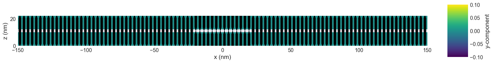

fig, ax = plt.subplots(figsize=(20, 6))
ax.set_xlim(-40,40)
ax.set_ylim(0,22)
system.m.sel("y").mpl(ax=ax, filename='../images/notebooks/mcut_init.png')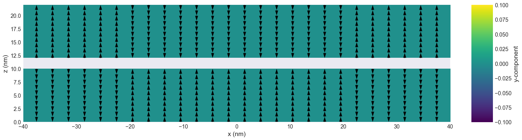

Simulation¶

Now we relax the system, in UberMag we use MinDriver to minimize the energy

md = oc.MinDriver()
md.drive(system)

OOMMFTCL is set, but OOMMF could not be run.
stdout:
b''
stderr:
b'couldn\'t read file "O:\\oommf\\oommf.tcl": no such file or directory\r\n'

Running OOMMF (ExeOOMMFRunner)[2025/06/03 13:06]... (63.0 s)

system.m.sel(z=17e-9).z.mpl.scalar(cmap='coolwarm')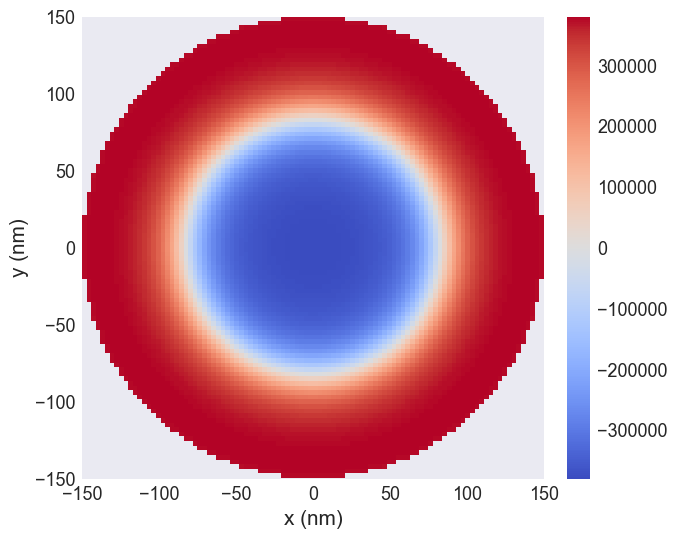

system.m.sel(z=5e-9).z.mpl.scalar(cmap='coolwarm')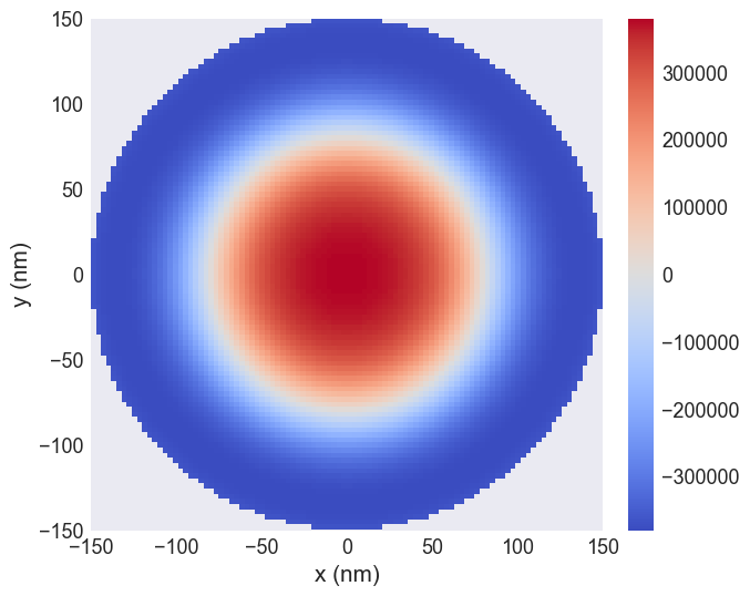

system.m.z.hv.scalar(kdims=["x", "y"], cmap='coolwarm')

fig, ax = plt.subplots(figsize=(20, 6))
ax.set_xlim(-50,50)
ax.set_ylim(0,22)
system.m.sel("y").mpl(ax=ax)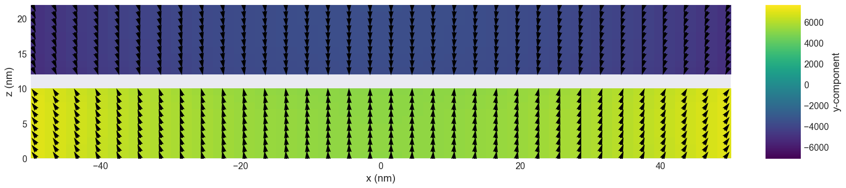

fig, ax = plt.subplots(figsize=(12, 8))
system.m.sel(z=17e-9).z.mpl.scalar(ax=ax, cmap="bwr", colorbar_label="z-component")
fig.savefig('../images/notebooks/skyrmion.png')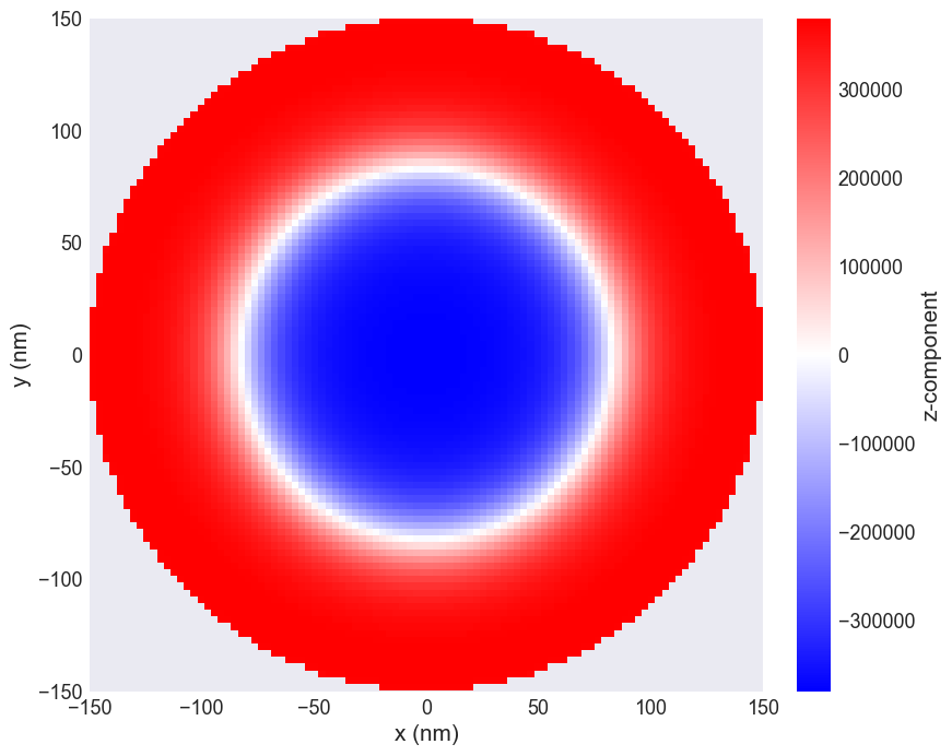

References¶

Batistel, T. M., & Brandão, J. (2023). Magnetic reversal stability of spin textures in synthetic antiferromagnetic nanodots. Journal of Magnetism and Magnetic Materials, 565, 170220. 10.1016/j.jmmm.2022.170220

Micromagnetics

Spintronics Neuromorphic

Micromagnetics

SAF Skyrmions Results